
Papers:

Papers:

Papers:

Papers:

Papers:

Papers:
Papers:

2025 Research Description: In 2025 the MathILy-EST topic was combinatorial representation theory, under the direction of Dr. Joshua Mundinger.
Combinatorics is the mathematics of counting. Often, objects we wish to count come with additional symmetry. Representation theory is the study of symmetries through linear algebra. Our projects will rely on the mutually beneficial relationship between combinatorics and representation theory: Representation theory can help combinatorics by turning a problem about sets into a problem about vector spaces, which are more flexible than sets; in turn, problems in representation theory may have answers in terms of nice combinatorial objects.
Here is how representation theory converts symmetries into linear algebra: If a set \(X\) has symmetries that form a group \(G\), the action of performing a symmetry on \(X\) can be described by a function \(G \times X \to X\). Then, a representation of \(G\) is a vector space \(V\) and such a function \(G \times V \to V\) such that \(g(v)\) is linear.
This summer, we will study combinatorics and representations associated to finite Coxeter groups. Coxeter groups are groups of symmetries of a vector space generated by reflections. For example, the group of permutations on three letters, \(S_3\), can be generated by reflections across the three lines shown in Figure 1. Each reflection corresponds to switching two letters. We write a permutation as disjoint cycles, where each cycle tracks how an element moves through the permutation; for example, \( (13)(2)\) means that the first and third elements switch places and the second element stays in its place.

Figure 1. Reflections across these lines generate \(S_3\); black permutations act on pink lists of numbers.

Figure 2. A Dyck path, traveling from corner to corner of an \(8\times 8\) grid staying above the diagonal, and corresponding non-crossing partition of the set \(\{1,2,\dots,8\}\). Their common permutation is \( (145)(23)(78)\).
A classic sequence in combinatorics is the Catalan numbers \(1, 2, 5, 14, 42,\dots\). There are at least \(214\) different kinds of objects all counted by the Catalan numbers, such as Dyck paths of length \(2n\) and noncrossing partitions of a set of size \(n\), both shown in Figure 2. It turns out that these Catalan objects are associated to the symmetric groups \(S_n:\) for example, each cell of a noncrossing partition corresponds to a cycle of a permutation (see again the example in Figure 2).
Amazingly, there are also Coxeter-Catalan objects associated to other Coxeter groups. We know lots about Catalan objects for the symmetric group, but comparatively less about Coxeter-Catalan objects. The known Coxeter-Catalan objects fall into two categories: nonnesting and noncrossing. Dyck paths are a nonnesting Catalan object, while noncrossing partitions are (surprise!) a noncrossing Catalan object. One question for this summer is: of those 214 known Catalan objects, which generalize to Coxeter-Catalan objects? Can we find new bijections between different Coxeter-Catalan objects? The Coxeter-Catalan objects can be interpreted in terms of representation theory, so we'll learn about representation theory to answer these questions.
Here's another place where combinatorics and representation theory meet. Instead of counting a single object, we can count several objects at once. A combinatorial species is a sequence of sets \(F_n\) labeled with \(\{1, 2, \dots, n\}\) where elements of \(S_n\), which are permutations, act by permuting the labels of \(F_n\). Part of an example is shown in Figure 3. On the combinatorics side, a combinatorial species has an associated generating function \(F(x) = \sum_{n \geq 1}|F_n|/n!\), which counts elements in \(F_n\) weighted by their symmetries. Many, but not all, operations of generating functions have analogous operations on combinatorial species. For example, under what conditions does the inverse function \(F^{-1}(x)\) count something? On the representation-theory side, we can use algebra and computer experimentation on a combinatorial species to study representations of \(S_n\).

Figure 3. Two members of the species of vertebrates (labeled trees with marked head and tail).
Combinatorial representation theory is a rich area with connections to many other parts of mathematics, and it deals with many concrete and beautiful objects (Catalan numbers, permutations,...). This summer, we'll get our hands on some of this great mathematics.
2025 Research Mentor: Dr. Joshua Mundinger is a Van Vleck visiting assistant professor at University of Wisconsin-Madison in Madison, WI. As an undergraduate, he participated in the SUNY Potsdam REU and several other undergraduate research projects. In 2022 he was an assistant mentor at MathILy-EST, guiding students in combinatorial representation theory. His research also involves algebraic geometry. In his spare time, he enjoys playing the piano.
2024 Research Description: In 2024 the MathILy-EST topic was combinatorial geometry of origami, an area that mixes discrete mathematics, geometry, and analysis, under the direction of Dr. Thomas Hull.
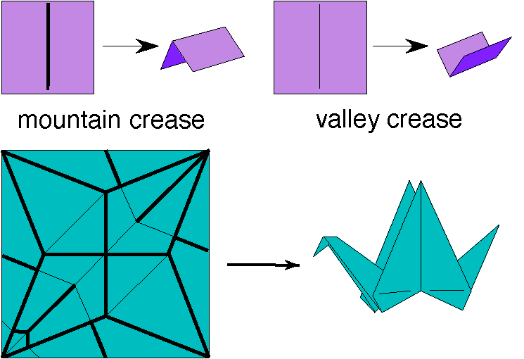
Crease and crease pattern examples
Origami is the art of folding paper, usually without making cuts, into interesting objects. Common to all mathematical studies of origami is the idea of a crease pattern, which is a planar graph \(C\) drawn on one's paper \(P\subset \mathbb{R}^2\) where the edges of \(C\), called creases, denote the folds made. Folded creases come in two types, mountains that fold away from your point of view and valleys that fold towards you. (Of course, flipping the paper over reverses all the mountain and valley creases.)
It turns out that understanding how origami works requires a mix of mathematical areas, and the problems we will undertake utilize aspects of geometry, combinatorics, and analysis. Many of these problems are motivated by applications, and this way of studying origami is relatively new in the world of mathematics.
A sample of the kinds of problems we will consider follows.
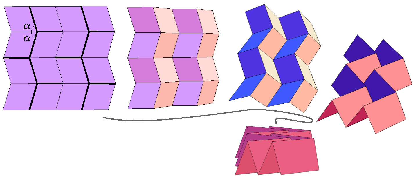
A rigid folding of the Miura-ori crease pattern
Origami has attracted the attention of physicists, engineers, and architects over the past 15 years. The intricate mechanics that rigid folding motions exhibit can be used in robotics and structure deployment. However, many open questions exist in the mathematics of such origami. A lot of progress on origami questions has been made in recent years, but many remain open, even for simple families of crease patterns.
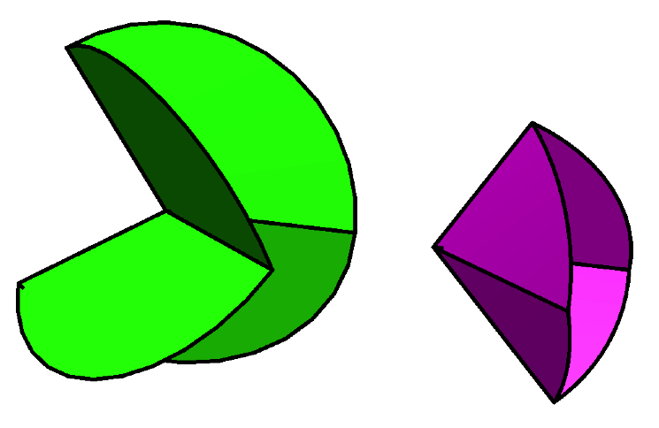
Vertices surrounded by more, or less, than 360 degrees of angle
2024 Research Mentor: Dr. Thomas Hull is an Associate Professor of Applied Mathematics at Franklin and Marshall College in Lancaster, PA. He has been researching the mathematics of paper folding since 1990 and is considered one of the world experts on the topic. He has written two books on the math of folding: the research monograph Origametry and the educational book Project Origami on using paper folding as a vehicle to teach math.
2024 Graduate Research Apprentice menTor at MathILy-EST (GReAT-EST): Natasha Ter-Saakov is a PhD student at Rutgers University specializing in combinatorics. As an undergraduate, Natasha studied mathematics (and computer science and education) at MIT. She participated in MathILy 2014 and 2015 and MathILy-EST 2019. When she is able to, Natasha enjoys fire spinning. At home, she can be found baking and even occasionally assembling IKEA furniture.
2023 Research Description: In 2023 the MathILy-EST topic was incidence geometry over finite fields, under the direction of Dr. Brian Freidin.
Given a polynomial \( f(x,y)\) in 2 variables, the line \( y=mx+b\) is tangent to the curve \( f(x,y)=0\) if the polynomial \( f(x,mx+b)\) has a repeated root, and otherwise the line is transverse to the curve. If multiple lines are tangent to a curve at the same point, the curve is called singular, and might involve a crossing or a cusp.
For instance, the curve shown at right, \( x^4-2x^3+x^2+xy+y^3-y^2=0\), is tangent to the green line at the green point because \( f(x,0)\) has a double root at \( x=1\). (Verify this by setting \( y=0\) and factoring.) The curve is also tangent to the orange line at the orange point because \( f(x,1-x)\) has a double root at \( x=0\). (Verify this by setting \( y=1-x\) and... ) And the curve is singular at the red \( (0,0)\) because it is tangent to every line \( ax+by=0\). (Verify this by...)
If we consider all our equations mod \( p\), basically setting \( p=0\), then we only have to think about points with coordinates between \( 0\) and \( p-1\). Similarly, we only have to think about lines and polynomials with coefficients in that same range. (And there are only finitely many possible lines!) In this setting, the curve\( f(x,y)=0\) is called transverse-free if it is tangent to every line that it intersects.
There has been some recent work counting the proportion of curves that are transverse-free, mostly focused on non-singular curves. This summer we will investigate the combinatorial and linear algebraic aspects of transverse-free curves. To include singular points, one goal is to understand the number of lines that avoid a given collection of singular points. The number of such lines, to which a transverse-free curve must be tangent, will vary depending on the number and placement of the singular points.
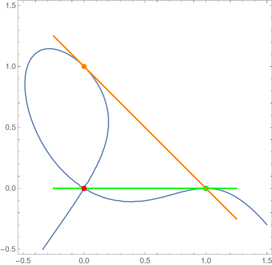
The curve \( x^4-2x^3+x^2+xy+y^3-y^2=0 \), along with two tangent lines and a singular point
In higher dimensions, given all the hyperplanes in \(n\) dimensional space mod \( p\), how many ways are there to select some points on each hyperplane at which a curve or surface should be tangent, so that no point is selected from more than one hyperplane? And if there are singular points, we need only select tangency points from the hyperplanes that avoid singularities.
Once we have selected some singular points and tangent hyperplanes, we can look for our transverse-free curves and surfaces. We can ask: How many polynomials \( f(x_1,\ldots,x_n)\) of degree \( d\) in \( n\) variables define a hypersurface \( f(x_1,\ldots,x_n)=0\) that is tangent to a fixed hyperplane \( a_1x_1+\cdots+a_nx_n=b\)? Fixing a point on the hyperplane, the condition of being tangent at that point imposes an equation relating the coefficients of \( f\) to each other. But if we want the hypersurface \( f=0\) to be tangent to several hyperplanes, or contain several singular points, how do the relations among the coefficients of \( f\) interact? How many hypersurfaces have all the tangencies and singularities we want to impose?
2023 Research Mentor: Dr. Brian Freidin is an Assistant Professor at Auburn University after earning a PhD from Brown University and a postdoc at the University of British Columbia. He did research as an undergraduate at the University of Illinois through the Geometry Lab and the Center for Complex Systems Research.
2023 Graduate Research Apprentice menTor at MathILy-EST (GReAT-EST): Lily Wang is a PhD student studying theoretical computer science at the University of Michigan. Her research interests are in combinatorics and graph theory. During her undergrad, she worked on research projects involving graph drawing, polytopes, and algorithm design. When she's not working, Lily enjoys hiking, art, and taking train rides.
2022 Research Description: In 2022 the MathILy-EST topic was combinatorial representation theory, under the direction of Dr. Nate Harman.
Algebraic objects are complicated. We can still gain insight by looking at oversimplifications: we will represent algebraic objects using matrices, so a representation is a collection of matrices that stand in for the algebraic object. Matrices are also linear functions, so they act on a vector space by transforming it.
Representation theory is the study of how algebraic objects such as groups and rings can be viewed geometrically as matrices acting on vector spaces. It is a fairly central field with direct connections to number theory, mathematical physics, logic, algebraic combinatorics, algebraic geometry, topology, and functional analysis.
One of the major triumphs of representation theory is that it often is able to reduce understanding complicated algebraic structures to (relatively) simple combinatorial structures. Combinatorial representation theory is the part of representation theory that engages directly with these combinatorial structures---often proving purely algebraic theorems using purely combinatorial arguments. Here is an example of one of the projects we will investigate this summer.
An irreducible representation is one that cannot be broken into smaller representations, so irreducible representations are the basic building blocks of all representations. Check out Figure 1 at right: it is a character tablefor the group \(S_5\), the collection of permutations of five elements. Algebraically, this table records the traces of matrices associated to group elements, with each row representing a different irreducible representation and each column representing a different kind of group element. Combinatorially the entries can be computed as an alternating sum over combinatorial objects called border-strip tableaux, an example of which is pictured in Figure 2 below.
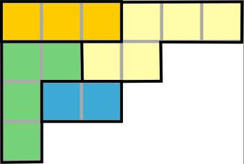
Figure 2: A small border-strip tableau.
Despite knowing how to compute these for over 80 years, recently some mathematicians began asking some pretty basic questions:
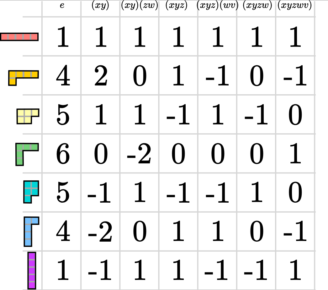
Figure 1: The character table for the symmetric group \( S_5\).
Some of these have simple answers. Others were only solved just in the last year or so. Others we still don't even know the answer to. This summer we will investigate some of these questions, as well as some generalizations. (Are there any other interesting patterns you notice or questions you have from looking at the table?)
2022 Research Mentor: Dr. Nate Harman is a postdoc at the University of Michigan after earning a PhD from MIT and stints at the University of Chicago and Institute for Advanced Study. As an undergraduate he participated in at least two REUs, and as a graduate student he mentored projects at the Research Sciences Institute and the MIT Program for Research in Mathematics, Engineering and Science for High School Students. Nate is also a player of board games, an eater of sandwiches, and a taker of naps. He is an avid fan of tacos, Batman, and hot sauce. He has run with the bulls (while participating in an REU!), jumped out of an airplane, and has spent many, many hours pretending to be a wizard.
2022 Graduate Research Apprentice menTor at MathILy-EST (GReAT-EST): Joshua Mundinger is a PhD student at the University of Chicago working in representation theory and geometry. As an undergraduate, he participated in several REUs. He is one of the organizers of the University of Chicago Mathematics Directed Reading Program, which coordinates independent reading projects for motivated undergraduates. He also is a pianist and loves to play chamber music.
2021 Research Description: In 2021 the MathILy-EST topic was discrete free boundary problems, under the direction of Dr. Max Engelstein.
Free boundary problems are a class of equations that often arise when some physically natural energy is minimized: every time you pull plastic wrap tight over a heaping plate of leftovers you solve a free boundary problem. Here, the edge of the plate is a fixed boundary, and the "free boundary" is where the plastic wrap comes detached from the pile of leftovers. See Figure 1.
This summer we will look at discrete versions of "Bernoulli" free boundary problems. We'll label each point of a square grid (more fancily, \(\mathbb Z^2\)) with a height, or more formally, let \(f: \mathbb Z^2 \rightarrow \mathbb R\). We model the energy by counting the grid points with positive height and adding the average squared difference in height between each pair of adjacent grid points. That gives us \[ E(f) = \#\{v\mid f(v) > 0\} + \frac{1}{4}\sum (f(v)-f(w))^2,\] (with 1/4 because each vertex has four neighborhoods). This energy function was originally proposed to model water cavitation, where the change in pressure from some quick motion causes bubbles.
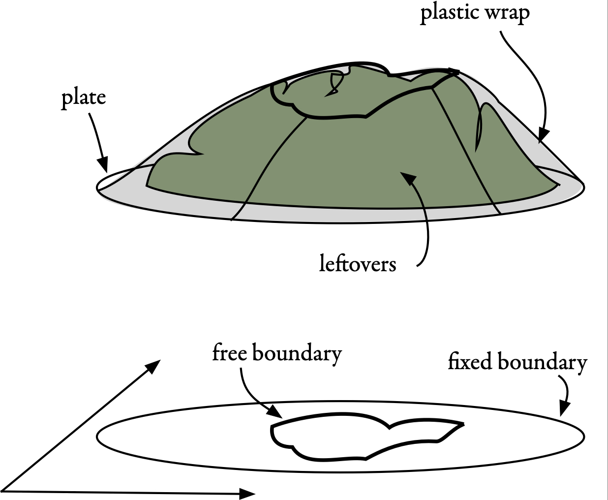
Figure 1: A plate of leftovers, with plastic wrap, fixed boundary, and free boundary shown.
Hugely simplifying, the first term represents the kinetic energy of the water flow and the second term takes into account the effects of pressure; the "free boundary" consists of points where \(f > 0\) that are adjacent to points where \(f = 0\) (this originally represented the interface between water and air). But we won't think much about water this summer---indeed, minimizers of a continuous version of \(E\) also have cool connections to random walks and eigenvalue problems; part of this project will be to see if these connections still exist in the discrete world!
A lot is known about the free boundary of critical points of the continuous version of \( E\) in the plane (see Figure 2 for some examples). But for the discrete problem there is still a lot to explore---what qualitative properties do these minimizers possess? Is the free boundary always connected or can it have lots of different components? Can the minimizing function alternate between positive and zero or does it switch precisely once? How do all these properties depend on the shape of the underlying grid (what if it is triangular or hexagonal as opposed to square)?

Figure 2: Critical points of continuous \( E \) are themselves functions. Here we have three examples of critical-point functions and their free boundaries.
2021 Research Mentor: Dr. Max Engelstein is an assistant professor of mathematics at the University of Minnesota in Minneapolis. As an undergraduate he participated in two REUs both of which are related to the current topic. Since then he has supervised undergraduate research projects as a PhD student at U Chicago and a postdoc at MIT. One of his main research interests is free boundary problems and he has published seven papers on free boundary problems related to the current REU topic. His interests lie at the intersection of two of the oldest subjects in mathematics: harmonic analysis and the calculus of variations.
2020 Research Description: In 2020 the research topic of MathILy-EST was sorting vertex labels on convex pieces of grids, under the direction of Dr. Hannah Alpert.
Ignoring the purple pentagon for a moment, we see in Figure 1 a graph with seven vertices and eight edges, along with two ways to number the vertices \(1\) through \(7\). We refer to these numberings as configurations, and we refer to the set of all \(7!\) configurations as a configuration space. We say that two configurations are adjacent, or one step apart, if they differ by swapping a set of disjoint pairs of numbers, with each pair sharing an edge of the graph; the configurations in Figure 1 are adjacent by swapping along the three teal edges.
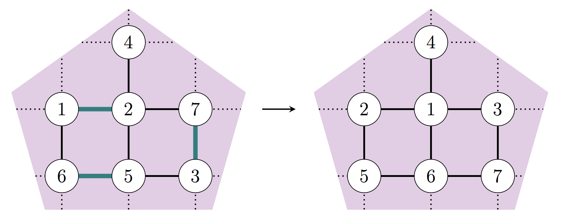
Figure 1: Two configurations have distance \(1\) if we can get from one to the other by selecting a set of disjoint edges and swapping the two numbers on each edge.
The distance between two configurations is the minimum number of steps needed to get from one to the other, and the diameter of the configuration space is the maximum distance between any two configurations.
The diameters of these configuration spaces have been studied for rectangular grids and for some other classes of graphs, but in this REU we will select graphs according to their geometric, rather than graph-theoretic, properties. In Figure 1 the graph is constructed by intersecting an infinite rectangular grid with the purple pentagon; we can consider all configuration spaces on graphs that are intersections of a rectangular grid with a polygon \(P\), focusing on the case where the grid boxes are very small relative to \(P\). When \(P\) is an arbitrary convex polygon in \(\mathbb{R}^2\), does the diameter of the configuration space behave roughly the same as when \(P\) is a rectangle aligned with the grid?
The geometric motivation is a continuous version of the problem: the configuration space of \(n\) disks of radius \(r\) in the polygon \(P \subseteq \mathbb{R}^2\) is the set of ways to arrange the disks, labeled \(1\) through \(n\), disjointly inside \(P\). In the REU, we will study discrete configuration spaces with the hope of finding properties that are also true of continuous configuration spaces.
2020 Research Mentor: Dr. Hannah Alpert is an NSF Postdoctoral Fellow in mathematics at the University of British Columbia in Vancouver, Canada. During her undergraduate years she participated in REUs every summer, and she is an author on six published papers on work she completed before entering graduate school. She first started working on questions related to the REU topic in 2014, with multiple related collaborations still ongoing, and her research interests lie more broadly within geometry and topology.
2019 Research Description: In 2019 the research topic of MathILy-EST was the combinatorics of flat origami, an area that combines discrete mathematics with geometry, under the direction of Dr. Thomas Hull.
Origami, otherwise known as paper folding, is modeled by a crease pattern \((P,C)\) where \(P\) is a compact region of \(\mathbb{R}^2\) (the paper) and \(C\) is a straight-line planar graph drawn on \(P\). A flat origami with crease pattern \((P,C)\) is a function \(f:P\to\mathbb{R}^2\) that is an isometry on every face of \(C\), continuous, and non-differentiable on the edges and vertices of \(C\).
Intuitively, flat origamis are folded paper models that can be pressed in a book without crumpling or adding new creases; see Figure 1 for some examples. We model how the faces of \(C\) get folded above or below neighboring faces via a mountain-valley (MV) assignment on the creases. Formally, a MV assignment is a function \(\mu:E(C)\to\{-1,1\}\), where \(E(C)\) is the edge set of \(C\) and \(-1\) denotes mountain (convex) crease while \(1\) denotes a valley (concave) crease.
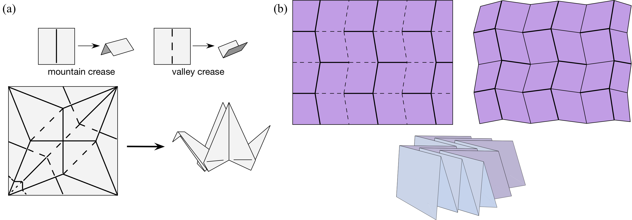
Figure 1: (a) Mountain and valley creases, with the classic crane crease pattern. (b) The Miura-ori crease pattern, with MV assignment, and the folded result.
A MV assignment is called valid if it can be realized in a flat origami \(f\) without causing any self-intersections of the paper. (For example, a crease pattern where all the creases are mountains would not be possible to fold flat, and thus is invalid.)
The major open problem in this area, which has applications in materials science and engineering, is the following: Given a flat-foldable crease pattern \(C\), how many different valid MV assignments exist on \(C\)? A recent advance has been the discovery that for some flat-foldable crease patterns this question can be translated into a graph-coloring problem. Developing a general theory of the link between valid MV-assignments and graph colorings (or other combinatorial structures) is the main thrust of this REU. Many smaller open problems exist, and will be explored, as we work towards this goal.
2019 Research Mentor: Dr. Thomas Hull is an Associate Professor of Mathematics at Western New England University in Springfield, MA. He has been researching the mathematics of paper folding since 1990 and is considered one of the world experts on the topic. His book Project Origami explores the use of origami in math education at the college level, and he is currently finishing Origametry: Mathematical methods in paper folding, a research-level monograph on origami mathematics forthcoming from Cambridge University Press.
MathILy, MathILy-Er, and MathILy-EST are projects of the nonprofit organization Mathematical Staircase, Inc..